PCA vs. ICA: Difference?

Here’s everything about the difference between PCA and ICA:

PCA tries to find mutually orthogonal components whereas in ICA the components may not be orthogonal.

ICA searches for mutually independent components. PCA tries to maximize the variance of the input signal along with the principal components, while ICA minimizes mutual information in found components.

So if you want to learn all about how exactly PCA and ICA differ, then you are in the right place.

Let’s dive right in!

PCA vs. ICA: Difference? (Coding Examples)

What Are the Basics of PCA and ICA?

PCA (Principal Component Analysis) and ICA (Individual Component Analysis) are based on similar principles, but still, they are different.

It isn’t easy to immediately understand all the formulas given when describing the PCA and ICA methods.

Mathematics is a beautiful science, but you need to go step by step to understand this beauty—it is almost impossible to jump several steps at once.

Often it is necessary to first investigate a particular method with a simple example so that you can form a picture in your head, which you can extend to more complex cases.

This is especially true in the case of multidimensional spaces such as the concepts of PCA and ICA.

The human brain cannot imagine an n-dimensional space for n > 3.

We will look at simple examples of PCA and ICA applications and try to understand the basic principles behind these methods.

Let’s start by setting a problem for the PCA:

What Is PCA and How to Implement It in Python?

Female writing on her notebook while looking at the laptop screen.

If we are talking about data analysis, then most likely you will use multidimensional feature arrays.

Such arrays, by the way, are called tensors.

It often happens that the dimension of this data is redundant. For example, one quantity may directly depend on another.

Let’s say you can calculate the square footage of an apartment from the square meterage of an apartment.

This means that we do not need to use both of these values in the analysis; you can discard one of the values (square footage or square meterage) in your analysis.

In this case, the correlation between the values is equal to one; that means they are strictly related.

But there may be weaker connections, for example, the acceleration time of a car from 0 to 100 mph depends on the engine size, but does not directly determine it.

There are other factors as well, such as vehicle weight and aerodynamics, engine design, and more.

If we know the exact formulas for the dependencies, then we can reduce the number of estimated factors, and merge them into one.

But of course, most often these dependencies are not so evident and difficult to find.

Nevertheless, some methods can reduce the dimension of the feature array for analysis.

One of these methods is PCA.

It allows you to select components from an array of features and assess how this or that component affects how strongly the real objects described by the studied features will differ from each other.

Let’s consider a synthetic example that will show how PCA works.

There may be many different PCA implementations.

We will model the simplest one.

To begin with, let’s take two values, they will depend on each other linearly, but additionally, let’s introduce a small random noise.

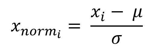
Let’s also standardize the values.

Subtract the expected value from each value and divide by the standard deviation:

%matplotlib inline
import matplotlib.pyplot as plt
import sklearn.decomposition as deco
plt.style.use('seaborn-whitegrid')
import numpy as np

x = np.linspace(1, 30, 100)
y = x + np.random.randn(100)

xnorm = (x - np.mean(x)) / np.std(x)
ynorm = (y - np.mean(y)) / np.std(y)

X = np.vstack((xnorm, ynorm))

Let’s transfer the points to the chart:

plt.plot(X[0], X[1], "o")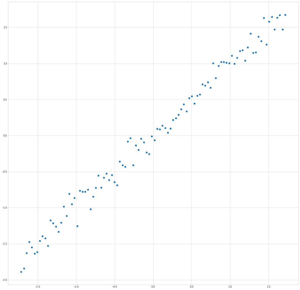

The graph clearly shows exactly what we put into the structure of the data, the dependence of the parameter y on x:

plt.plot(X[0], X[1], "o")
plt.plot([-2,2], [-2,2])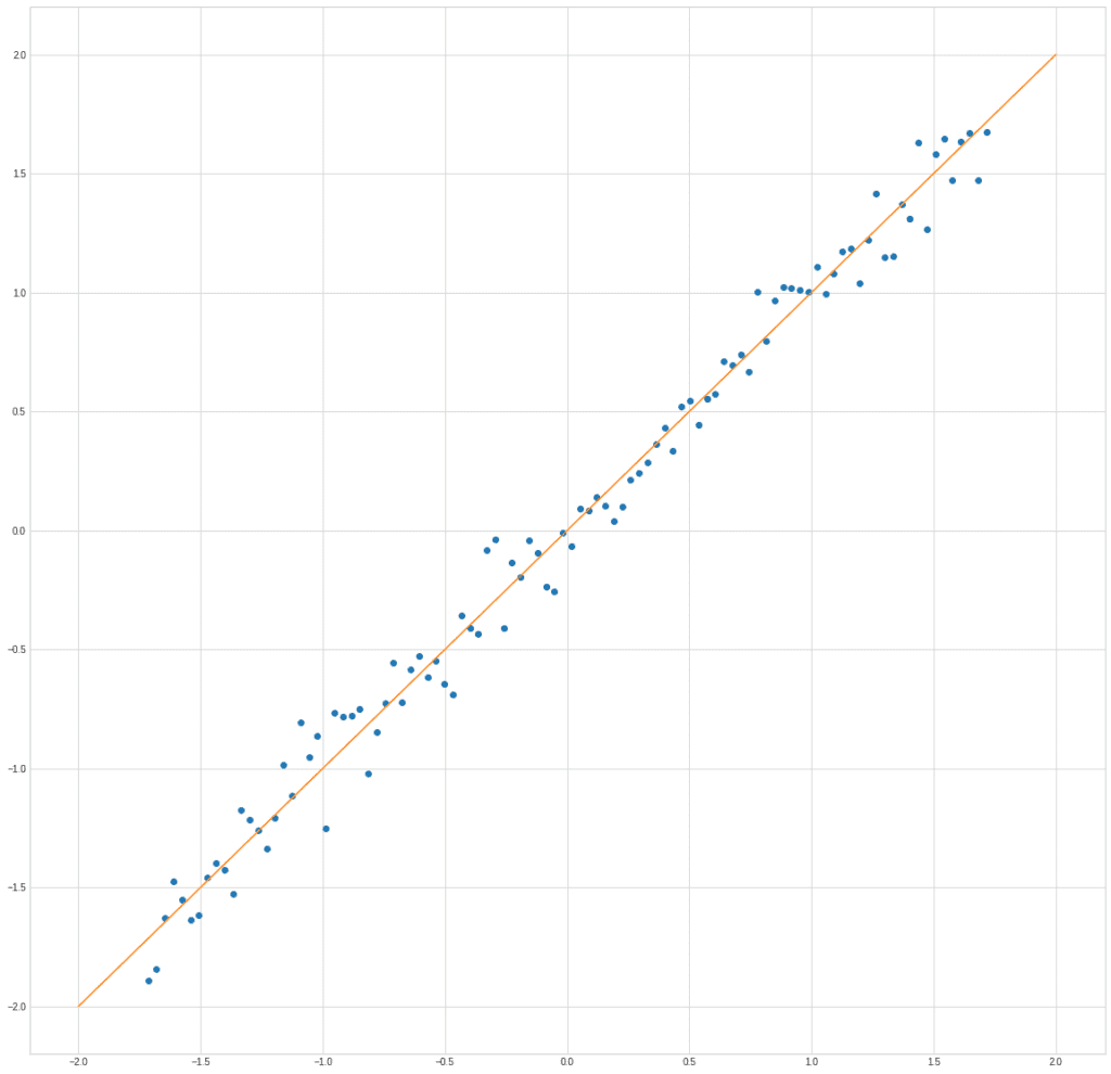

With the help of PCA, we can find a new trait that will be a combination of the two.

Naturally, when replacing two features with one, some information will be lost.

The task of the algorithm is to minimize these losses.

In this case, you can obviously use the projection of points on the line x1 = x2.

It is along this line that the data spread is maximal.

We use a covariance matrix to estimate the dependence of two vectors.

Covariance is generally defined as a measure of the dependence on two random variables:

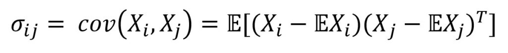
Where E is the expectation operator. So, we center the vectors—subtract the mathematical expectation of the vector from each value, and then find their inner product.

The scalar product in Euclidean space is defined as the product of the vector lengths by the cosine of the angle between them.

If the vectors are orthogonal, then the cosine of the angle will be 0.

Accordingly, calculating the dot product, we are looking for how much the vectors do not coincide in direction.

The variances of the corresponding values are located along the principal axis of the covariance matrix. It is easy to find the covariance matrix in python.

For the signs, it will be like this:

covariance = np.cov(X)

print(covariance)

[[1.01010101 1.00366207]
 [1.00366207 1.01010101]]

What will the covariance matrix look like?

It will look diagonal.

Apart from the main diagonal, the rest of the values will be zero.

We are just trying to find such a basis, that is, we need to diagonalize the covariance matrix.

This is easy to do with eigendecomposition.

We can represent any square matrix of linearly independent rows as:

Where Q is a matrix consisting of eigenvectors, and Λ is a diagonal matrix, the elements of which along the main diagonal are equal to the eigenvalues of matrix A, and the other elements are equal to 0.

Thus, to find a new basis—vectors along which the dependence will be minimal, we must find the eigenvectors of the covariance matrix.

And that’s easy to do with the NumPy module too:

eigenvalues, eigenvectors = np.linalg.eigh(covariance)

print(eigenvectors)
print(eigenvalues)

[[-0.70710678  0.70710678]
 [ 0.70710678  0.70710678]]

print(eigenvalues)

[0.00642988 2.01377214]

The vectors themselves are located in the columns of the resulting matrix. Let’s select the first and second eigenvectors for the covariance matrix:

ev1 = eigenvectors[:, 0]
ev2 = eigenvectors[:, 1]

We can check that they are indeed eigenvectors by definition.

The product of a matrix by an eigenvector must be equal to the product of an eigenvalue by the same vector:

print(covariance @ ev1)
print(eigenvalues[0] * ev1)

[-0.00455302  0.00455302]
[-0.00455302  0.00455302]

print(covariance @ ev2)
print(eigenvalues[1] * ev2)

[1.42394553 1.42394553]
[1.42394553 1.42394553]

As you can see, the result is identical.

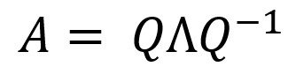
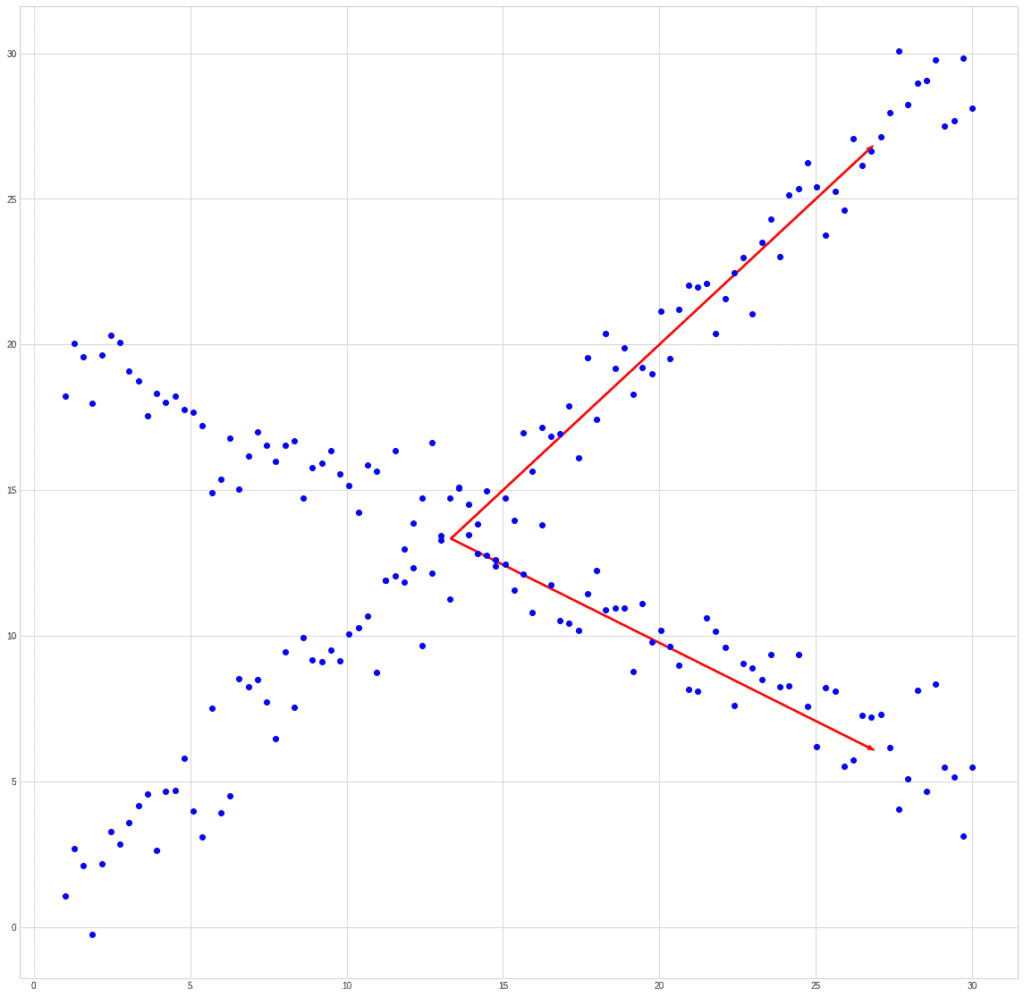
Let’s try to plot the vectors along with the data set to make sure we actually found the right directions:

plt.plot(X[0], X[1], "o")
plt.arrow(0, 0, ev1[0] * eigenvalues[0] * 10, ev1[1] * eigenvalues[0] * 10, color = "r", width = 0.01)
plt.arrow(0, 0, ev2[0] * eigenvalues[1], ev2[1] * eigenvalues[1], color = "b", width = 0.01)
plt.show()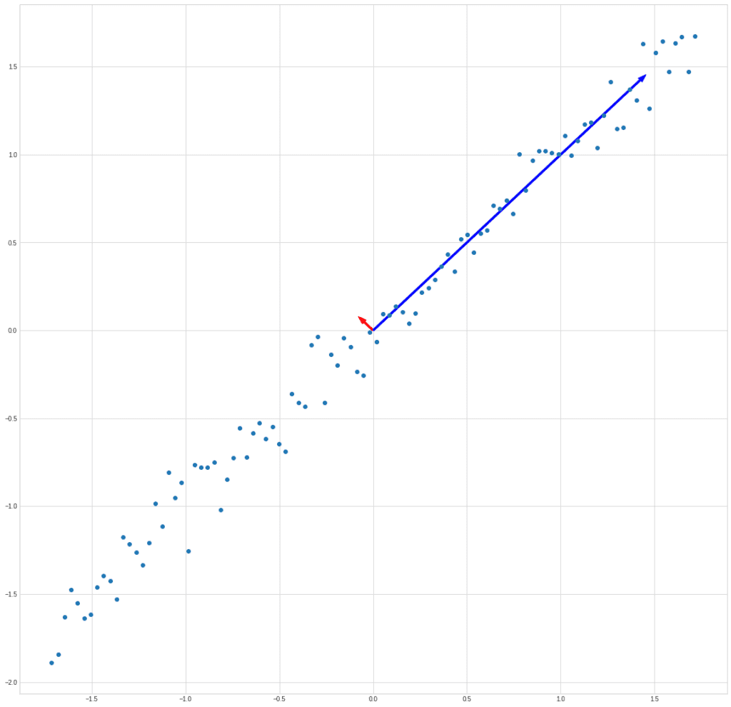

We draw the vectors not to scale because the eigenvalues in the example differ by 4 orders of magnitude.

But we see that we have got two orthogonal vectors, one of which is directed towards the maximum dependence, and the other is perpendicular to it.

To get the new coordinate values, we just have to multiply the matrix of eigenvectors by the original matrix of features:

X_new = eigenvectors @ X

Now let’s find the standard deviation of the two new features:

print(np.std(X_new[0]))
print(np.std(X_new[1]))

0.07984079617577441
1.4119580189460372

The standard deviation along the axis of the red vector is 17 times less than along the blue one. We can discard the entire column and use only one X_new [1] instead of two features x1 and x2.

In fact, it turns out that we are replacing the blue dots with green ones:

plt.plot(X[0], X[1], "o")
plt.plot([-2,2], [-2,2])
plt.plot(X_new[1] / np.sqrt(2), X_new[1] / np.sqrt(2), "o")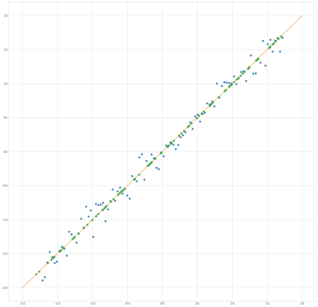

Of course, there are losses, but in many cases, they can be neglected.

It is possible to calculate the loss of information by evaluating the ratio of the eigenvalues that remain and those that we discard.

In general, PCA allows you to transform n features into m, where m << n.

For practical tasks, it is more convenient to use ready-made implementations.

For example, we can take the PCA model from the sklearn.decomposition module:

from sklearn.decomposition import IncrementalPCA

X = np.stack((xnorm, ynorm), axis = 1)
pca = deco.PCA(1)
xt = pca.fit_transform(X)

print(xt.shape)

(100, 1)

We pass one parameter to the deco.PCA function—m, the new number of features that we want to keep.

At the output, we get an array of new features, some of which are automatically discarded in accordance with the specified parameter.

We can compare the features calculated by the method and the finished function from sklearn:

printzip(* (xt.reshape(100), X_new[1]))

(-2.378511170140015, -2.3785111701400123) 
(-2.4911929631729186, -2.4911929631729177) 
(-2.172690411576331, -2.1726904115763306) 
(-2.321844756744973, -2.3218447567449725) 
( -2.213965105057678, -2.213965105057677) 
(-2.0648350319020237, -2.0648350319020228)
...

The output is truncated to the first 6 pairs of numbers. As you can see, they match up to the rounding error.

What Is ICA and How to Implement It in Python?

You can hear about ICA most often as a way to solve the blind source separation problem.

This problem is also called the cocktail party problem.

Imagine that you are at a party where several dialogues take place at the same time.

It is quite noisy around you, but you can still communicate with the interlocutor, the human ear and brain successfully solve this problem and isolate the significant signal from the general noise.

The solution to this problem is not so simple mathematically:

Let’s imagine that we have 3 signal sources and several microphones that record a linear combination of signals.

The number of microphones must be no less than the number of signal sources. Otherwise, the task will be undefined.

Also, for the task to make sense, signals have to meet two requirements:

Signal sources are independent of each other;
The values of each of the sources have a non-Gaussian distribution.

The signal sources are independent, but their mixtures are, of course, not independent, since each of the mixtures depends on all sources.

But the more sources we have, the closer the distribution of each mixed signal will be to Gaussian.

This is where the separation is based; we will try to isolate the most non-Gaussian components from the mixed signals.

In any implementation of the ICA algorithm, We can distinguish three stages:

Centring (subtracting the mean and creating a zero mean for the signal)
Removing from the correlation (usually using the spectral decomposition of the matrix)
Reducing the dimension to simplify the problem

If we try to compare PCA and ICA using the past example, then we get something like this. Let’s take a mixed signal:

PCA will find the vector in the direction of which the variance is maximum.

ICA will find vectors corresponding to the mixed signals.

This example is synthetic.

You should understand that the limitation of ICA is that it cannot restore the order of the original signals, as well as their actual amplitude.

But this is not a problem for tasks such as splitting audio signals, for example.

Let’s try to mix and split two images from Unsplash:

from matplotlib import image

s1 = image.imread("s1.jpg")
s2 = image.imread("s2.jpg")

plt.imshow(s1)

plt.imshow(s2)

Create blended images and normalize them so that the brightness values stay in the range 0…255:

m1 = 0.6 * s1 + 0.4 * s2
m2 = 0.3 * s1 + 0.7 * s2

norm = lambda x: (x * 255 / np.max(x)).astype(np.uint8)

m1 = norm(m1)
m2 = norm(m2)

plt.imshow(m1)

plt.imshow(m2)

As you can see, these blended images are similar to it as if you were looking at something through the glass and saw partly the picture behind the glass, and partly the reflected image.

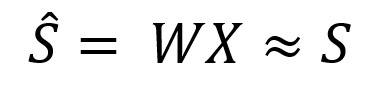
Our task now is to find the matrix W. Such that multiplying this matrix by the input matrix of mixed signals will give us approximately the matrix of the original independent signals:

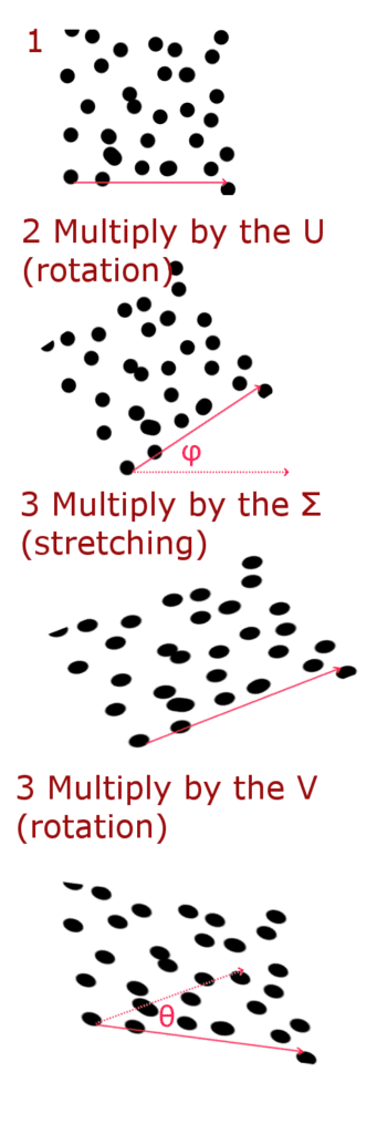
We can solve this problem through SVD (Singular Value Decomposition). We represent the desired matrix as:

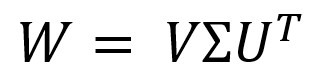
Where Σ is a diagonal matrix, which can be represented as a stretching (scaling) matrix, and the U and V matrices are rotation matrices.

You can write a rotation matrix in this way—this matrix will rotate a vector for an angle θ when multiplying:

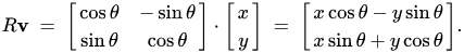
Thus, we can represent multiplication by the matrix W in 3 stages:

Now let’s implement it in Python. The derivation of formulas are not described in detail. You can see them in the source.

Find θ and see its value in degrees:

theta0 = 0.5 * np.arctan(-2 * np.sum(m1 * m2) / np.sum(m1 ** 2 - m2 **2))
theta0 * 180 / np.pi

-31.781133720821153

Further find transposed matrix U:

Us = np.array([ [np.cos(theta0), np.sin(theta0)], [-np.sin(theta0), np.cos(theta0)] ])
Us

array([[ 0.85006616, -0.52667592],
       [ 0.52667592,  0.85006616]])

And the matrix Σ:

sigma1 = np.sum( (m1 * np.cos(theta0) + m2 * np.sin(theta0) ) ** 2)
sigma2 = np.sum( (m1 * np.cos(theta0 - np.pi / 2) + m2 * np.sin(theta0 - np.pi/2) ) ** 2)
Sigma = np.array([ [1/np.sqrt(sigma1), 0], [0, 1/np.sqrt(sigma2)] ])
Sigma

array([[9.39029733e-06, 0.00000000e+00],
       [0.00000000e+00, 2.15484602e-06]])

Let’s multiply the mixed signals by the known matrices U and Σ and calculate the angle φ:

x1bar = Sigma[0][0] * (Us[0][0] * m1 + Us[0][1] * m2)
x2bar = Sigma[1][1] * (Us[1][0] * m1 + Us[1][1] * m2)

sum1 = np.sum(2 * (x1bar ** 3) * x2bar - 2 * (x2bar ** 3) * x1bar)
sum2 = np.sum(3 * (x1bar ** 2)* (x2bar ** 2) - 0.5* (x1bar ** 4) - 0.5 * (x2bar ** 4))

tmp1 =  -sum1 / sum2
phi0 = 0.25 * np.arctan(tmp1)

phi0 * 180 / np.pi

-1.7576366868809685

Form the matrix V:

V = np.array ([ [np.cos (phi0), np.sin (phi0)],
 [-np.sin (phi0), np.cos (phi0)] ])

V

array([[ 0.99952951, -0.03067174],
       [ 0.03067174,  0.99952951]])

Let’s calculate the signal values, normalize them and display the images on the screen:

s1hat = V[0][0] * x1bar + V[0][1] * x2bar
s2hat = V[1][0] * x1bar + V[1][1] * x2bar

s1hat = norm(s1hat).astype(np.uint8)
s2hat = norm(s2hat).astype(np.uint8)

plt.imshow(s1hat)

plt.imshow(s2hat)

As you can see, the images recovered pretty well. Although not perfect—you can see the noise and outlines of past images.

What Are the Similarities and Differences Between PCA and ICA?

We have looked at the Python implementations of PCA and ICA.

Now let’s talk a little about the similarities and differences:

Similarities:

Both of these methods are statistical transformations
Both of them are widely used in various applied problems, often even in the same ones
Both methods find new bases for representing input data
In both cases, we consider that the observed features are a linear combination of certain hidden features
Both methods assume that the components are independent and have a non-Gaussian distribution

Differences:

PCA tries to find mutually orthogonal components; in ICA the components may not be orthogonal. ICA searches for mutually independent components
PCA tries to maximize the variance of the input signal along with the principal components, ICA minimizes mutual information in found components.
The features obtained in the PCA are in strict order from most significant to least significant. Therefore, we can discard some of the features to reduce the dimension. Components obtained in ICA are fundamentally unordered and equivalent. We cannot sort them.

What Are the ICA and PCA Applications?

You can use ICA to remove various kinds of “noise.”

Including noise in the image, as well as the removal of certain objects from the input data set.

For example, you can remove the eye blinking from the electroencephalogram data. ICA is also used for time series analysis to identify “trends”.

This can be applied in predicting prices in the stock market or in analyzing trends in social media posts.

Downsizing data with PCA can be used to visualize data.

You cannot plot points in ten-dimensional space on the two-dimensional plane of the screen.

PCA can also be used to compress videos and images.

You can use PCA to suppress noise in images.

PCA is also widely used in:

Bioinformatics
Chemometrics
Econometrics
Psychodiagnostics

Author

Theresa McDonough

Tech entrepreneur and founder of Tech Medic, who has become a prominent advocate for the Right to Repair movement. She has testified before the US Federal Trade Commission and been featured on CBS Sunday Morning, helping influence change within the tech industry.

View all posts